VLOOKUP Function
VLOOKUP in Excel is a premade function that searches for a specified value vertically across a table array or column range. Once it locates that value, it can then retrieve and return associated data/information with that value.
Use the VLOOKUP in Excel or Google Sheets to quickly find an exact match or approximate match in a table array, range, or large spreadsheet. You can quickly find, sort, and interpret data accurately with it.
VLOOKUP Explained Step By Step
“V” in the VLOOKUP stands for “vertical,” ー altogether implying ー “vertical lookup” (vertical search)
Excel VLOOKUP function means the action of looking up information vertically across a spreadsheet’s column(s). After locating the value in the first column of the spreadsheet ー using a unique identifier as a basis for the search in the column(s) to its right, ー finds and returns a piece of information (return value) associated with that value from the first column within the same row.
VLOOKUP Formula
The VLOOKUP function (VERTICAL LOOKUP) formula is typed =VLOOKUP(lookup_value, table_array, col_index_num, [range_lookup]).
Which denotes,
=VLOOKUP[lookup_value, table range starting from the column containing the lookup_value to its right, the column number in the specified range in which the return corresponding value is, specify whether to look for a True(Approximate match) or Exact match (FALSE)]
The VLOOKUP works to help organize data in such a way that the lookup value is to the left of the return value you want to find.
VLOOKUP Syntax Explained
The VLOOKUP function contains 4 arguments, of which the first three out of four arguments of the VLOOKUP formula are mandatory, and the last or 4th is an optional argument.
Note: Arguments in an Excel function can be various types of data, such as numbers, text, logical values (like TRUE or FALSE/approximate match or exact match ), table array, error values (like #N/A), column number, or cell references. These arguments can also be constants, formulas, or even other functions.
The 4 arguments that make the VLOOKUP signify:
First argument/lookup_value: This is a mandatory parameter that signifies the value searched for in the first column number of a dataset column or table array to be selected.
Second argument/table array: This is also a required parameter that denotes the table array or table range of columns that contains both the lookup values and the results.
Third argument/column index number: This is a compulsory parameter that indicates the integer that specifies the column number or column index number in the specified table array.
Fourth argument/range lookup: The fourth argument of the VLOOKUP function is a Boolean expression. This is an optional parameter that determines whether the function should return an exact match or an approximate match for the lookup value. This argument can be set to either “FALSE” or “TRUE.”
NOTE: Boolean expressions are statements that use logical operators to evaluate a condition and result in a Boolean value, i.e., true or false/1 or 0/approximate matches or exact matches.
- Fourth argument being ‘TRUE’ suggests an approximate match (if an exact match isn’t found, it uses the closest match below the lookup value).
- Fourth argument being While ‘FALSE’ suggests an exact match (if an exact match isn’t found, it returns an error).
VLOOKUP Function Always Searches To The Right
While using the VLOOKUP function in Excel, you’re looking for new information in a different column that is associated with known data in the first column of the table array. When the VLOOKUP function runs this search, it always looks for the new information to the right of your known data.
VLOOKUP Function Needs The Unique Identifier To Retrieve A Result
A unique identifier, as the name suggests, is a distinctive piece of data that is common to both of your data sources(known and unknown).
The VLOOKUP function uses the “Unique Identifiers” to identify the result correctly.
It’s unique in the sense that it corresponds to only one entry in your database. Examples of unique identifiers are product codes, stock-keeping units (SKUs), and customer contacts. These identifiers are exclusive to each record, ensuring precise data retrieval.
VLOOKUP Function’s Working in Layman’s Terms
The VLOOKUP function basically operates similarly to a phone directory, allowing the use of a known data point, such as a person’s name, to find an unknown piece of information, like their phone number or address.
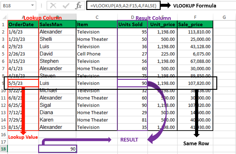
The VLOOKUP function is basically used when you have a known value(lookup value) ー from the first column (lookup column) of any selected table range or spreadsheet (table array) ー and you need to find an corresponding value(result) ー from a corresponding column (result column) with the help of a unique identifier from the same row.
How do you find an exact match using the VLOOKUP Function?
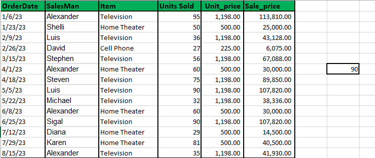
Excel VLOOKUP function can find the exact match efficiently from a table. To find an exact match using VLOOKUP in Excel, set the lookup value, table array, column index (e.g., 4), and the fourth argument to False. For example, VLOOKUP(A9, A2, 4, FALSE) will return 90 if the exact match is found.
Follow the process explained below with an example to learn how to find an exact match:
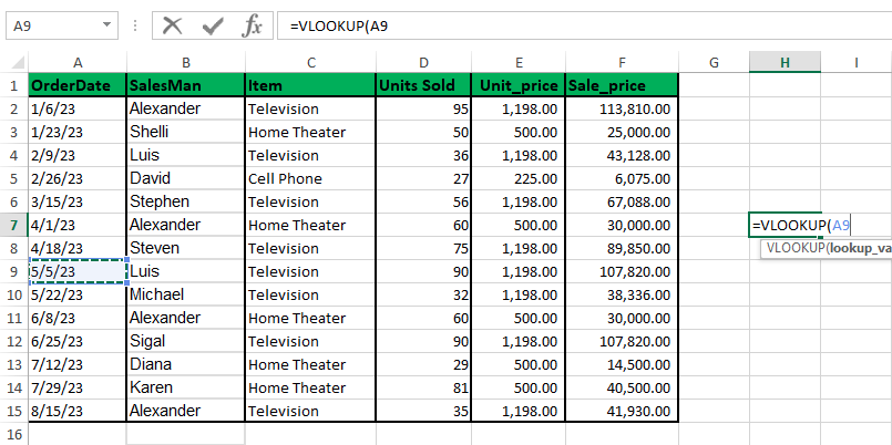
Here, from the database below, we need to find the units sold on the date 5/5/23 by using the VLOOKUP function. So, we set the first parameter as cell A9, which is the lookup value.
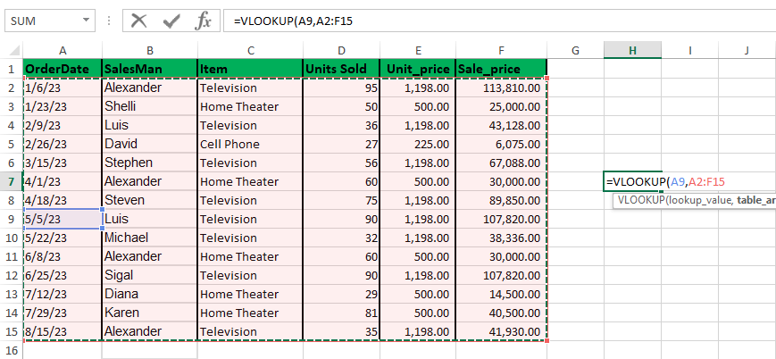
Now, we select the range of the table array where the desired value lies in the second argument of the VLOOKUP function. Here, the table array is A2:F15.
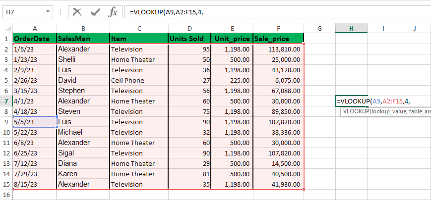
We need to specify the Column Index Number for the third argument, which is 4 in this case. This VLOOKUP function argument should point out the column in which the cell we are looking for exists. The lookup value and the return value always exist in the same row in case of finding exact matches.
The fourth argument of the VLOOKUP function is a Boolean expression as discussed earlier. We will set the value to False for the fourth argument to find an exact match of the lookup_value.
Note: N/A error will be displayed in case the exact value is not found or if the VLOOKP function is entered incorrectly.

Press enter to get the result, which in our case is 90.
How do you find an approximate match using the VLOOKUP Function?
The approximate the match function of the VLOOKUP function works by locating the next largest value that is lesser than the lookup value we provide.
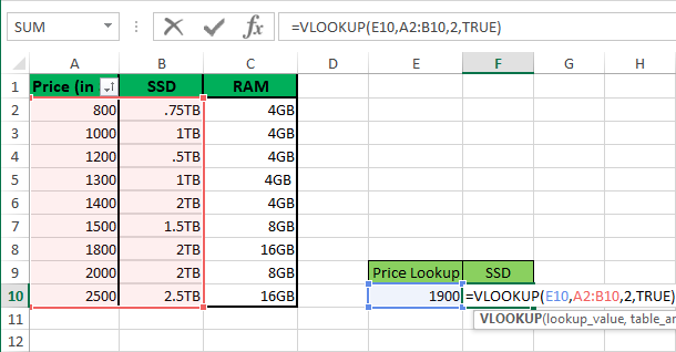
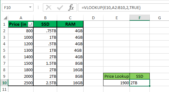
In the following example, we will use the VLOOKUP in Excel to find out an approximate match of how much SSD specification a laptop priced at $ 1900$ would have. Also, we are aware that this value is not present in the table array.
First, specify your lookup value. Here, the lookup value is $1900.
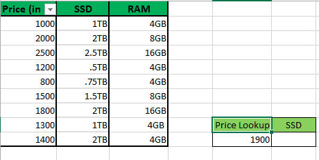
To begin, we will now sort the first column in ascending order using the Filter Option. If not, the VLOOKUP function will malfunction and return no or wrong value.
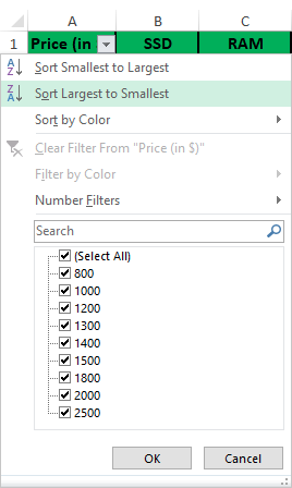
Next, select the data array and select the filter option to sort the values of the first column.

Filter the price details in ascending order. Click on OK.
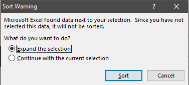
Choose the option to expand the selection and press Sort.
Now, input your VLOOKUP function. The first parameter is the lookup value(1900 or E10) from the first column number. The second parameter defines the lookup table array in range(A2:B10). The third parameter is the column index number (2) from which values will be retrieved. Lastly, the final parameter is set to TRUE, enabling the VLOOKUP function to locate an approximate match.
Once the VLOOKUP function is entered, hit enter.
The returned value in this scenario is 2TB for a price of $1900.
How to Use VLOOKUP Across Multiple Sheets
Use VLOOKUP across multiple sheets in Excel, open both worksheets, identify a common field, enter the VLOOKUP formula with correct parameters, and press Enter to retrieve the data.
Follow the following steps to apply the VLOOKUP function across multiple worksheets:
1. Access the Worksheets
Open the worksheet that contains the data you need to find, as well as the worksheet where you intend to display the lookup results.
2. Identify the Common Field
Find a common field in both worksheets that will serve as a reference for your lookup. This could be a unique identifier like a product serial number or a customer code.
Note: Make sure that the common reference field in both worksheets aligns correctly.
3. Enter the VLOOKUP Formula
In the worksheet where you want the lookup results to appear, input the VLOOKUP formula into the cell where you want the data to be displayed.
4. Specify the Parameters in the Formula
Within the VLOOKUP formula, define the lookup value, the cell range in the source worksheet where the lookup values can be found, the column index number of the data you want to find, and the cell range that contains the source data across multiple sheets. These arguments should be separated by commas.
5. Execute the Formula
Press Enter to execute the VLOOKUP function, and the lookup result will appear in the designated cell reference.
How To Fix VLOOKUP Function Not Working?
If VLOOKUP isn’t working, check the syntax for accuracy: verify the lookup value, table array, sheet references, column index, and fourth argument. Also, ensure values are correctly formatted and aligned.
Follow the step-by-step information given below:
- Your VLOOKUP syntax (structure of the formula)
- Values (the quality/ accuracy/ formatting of the data in the formula).
VLOOKUP Syntax Troubleshooting
Cross-check the formula for VLOOKUP in the cell and check for the following pointers:
- In reference to the unique identifier, is the lookup value accurate?
- Does it define the right table array range for retrieving values(should contain the lookup value and where the result may exist)?
- Is the sheet specified correctly?
- Is the syntax for referring to the sheet correct?
- Is the column index number or column number correct?
- Is the fourth argument/ last argument (True or False) given appropriate for your sheet setup?
Value Troubleshooting
If the VLOOKUP syntax isn’t the problem, the issue might be with the values you’re trying to retrieve. This often results in an #N/A error when VLOOKUP can’t find a referenced value. Check whether;
- If values are formatted vertically?
- Is the table array starting from the lookup column to its left or not?/ Is the lookup value in the left most column or not?
- If the values are specified accurately?
For instance, if you’re looking up Sales data, each Sale detail should be a row with its related data to its left in the same row. If the Sales details are column headers with vertical data, VLOOKUP won’t work. In reference to use VLOOKUP across multiple sheets, the Sales data must match in format in both sheets respectively.
Takeaway
The VLOOKUP formulas in both EXCEL and GOOGLE SHEETS are great assets that can be leveraged to manage multiple spreadsheets. Use the VLOOKUP function to analyze and find data/information from a variety of sources to get a complete picture and accurate information for tasks like lead generation, finding sales records, accounting, and more.
With the help of the above guide for the VLOOKUP function, you can easily understand its functioning and how it’s used, find Exact/Approximate matches across single or multiple worksheets accurately.
Frequently Asked Questions
What is VLOOKUP Function?
VLOOKUP function searches that vertically searches for a specified value in the first column of a table and returns a corresponding value from another column in the same row as per the given arguments.
Does the VLOOKUP Function Supports Searching for a Value Horizontally?
No, the VLOOKUP returns value for vertical search only. For horizontal searches, use the HLOOKUP function.
What is the Range Limit for the VLOOKUP Function in Microsoft Excel?
VLOOKUP Excel function can search up to 1,048,576 rows, the maximum number of rows in an Excel worksheet.
Can VLOOKUP Work With Multiple Worksheets?
Yes, VLOOKUP can work across multiple worksheets in the same workbook. You can include the sheet name and cell range in the table_array argument of the VLOOKUP function.
How Can I Avoid Errors With VLOOKUP?
To avoid VLOOKUP errors, ensure the lookup value is in the first column, verify the column index number, use the [range_lookup] parameter correctly, and handle errors with the IFzERROR function.
To prevent errors and make sure VLOOKUP returns the desired specific value, make sure:
- The lookup_value is in the first column of the table range selected not in the third column or any else.
- Verify that the col_index_num (numeric value) refers to the right column for the data you want.
- Be careful when using the [range_lookup] parameter for exact or approximate match as it can give unexpected results.
- Use the IFERROR function to handle possible #N/A errors smoothly.
- The data in the context table_array must be organized in columns.
Will the Functioning of VLOOKUP be Affected by the Letter Casing of Values in Reference Cells?
The VLOOKUP function identifies both upper case and lower case letters as equal. For example, the function will see the term “TEXT” as the same as “text.”
